Langevin Sampling: Discretization Bias and Transport Coefficients

by Akshat Valse

Advised by Dr. David Herzog, Department of Mathematics, Iowa State University

We study what a Langevin sampler loses when it drops the Metropolis step (ULA), and what keeping the step (MALA) does not fix. On a Gaussian target, ULA’s invariant law is known exactly, with an excess variance first order in the step size, and the measured variance lies within three standard errors of it in all 30 cases. MALA removes the bias, but on a two-well mixture its crossing rate still falls roughly exponentially with the barrier. Live figures check the dynamics too, against the Lifson–Jackson effective diffusivity.

Code Demo

Draft in Advisor Review

A flat contour map of two wells seen from above: a dark purple figure-eight runs diagonally across the frame, its two lobes touching at a single point, with warm bands of coral, pink, peach and apricot rippling outward to cream at the corners.

Introduction

A Langevin sampler discretizes a diffusion whose invariant law is the target. Stochastic-gradient Langevin dynamics, the inner loop of annealed Langevin sampling and the corrector step of a predictor–corrector diffusion sampler all run the same Euler–Maruyama update, and none of them performs the accept/reject test that would make it exact in stationarity. That mapping is this site’s framing: the repository behind this page tests only the two textbook samplers, the unadjusted Langevin algorithm (ULA) and its Metropolis-adjusted version (MALA). Skipping the test, or keeping it, raises two separate questions:

Discretization bias (what skipping the test costs): ULA’s invariant law differs from the target. On a Gaussian target that law is known exactly, so we grade the simulation against the answer rather than against a longer run of itself, and a failure would convict the sampler rather than the theory.
Slow mixing (what keeping the test does not fix): MALA is unbiased, but only in stationarity. On a separated two-well target, does it get there any faster than ULA?

We answer both with the repository’s saved runs, then turn from the invariant law to the dynamics, which this site’s live figures check against the classical Lifson–Jackson effective diffusivity.

The project began in May 2026 and is advised by Dr. David Herzog, Department of Mathematics, Iowa State University. It has a public part and an unpublished one. The public part, the langevin-samplers repository and this site’s live figures, is reported here with its results. The unpublished part is a manuscript with Dr. Herzog on transport-coefficient estimation for molecular systems, now drafted and in his review; its section says what it is about, and its results are held back pending submission.

Two Samplers and an Exact Reference

Both samplers make the same move; MALA may then reject it. Let $\pi$ be a target density on $\mathbb{R}^d$ with score $\nabla\log\pi$ . The overdamped Langevin diffusion

dX_t = \nabla \log \pi(X_t)\,dt + \sqrt{2}\,dW_t

leaves $\pi$ invariant, so discretizing it gives a sampler. With step size $h>0$ and $\xi_k \sim \mathcal N(0, I)$ i.i.d., its Euler–Maruyama discretization is ULA,

X_{k+1} = X_k + h\,\nabla \log \pi(X_k) + \sqrt{2h}\,\xi_k ,

whose invariant law $\pi_h$ generally differs from $\pi$ . That gap is the discretization bias. MALA uses the same move as a proposal $y$ and accepts it with probability

\alpha(x,y) = \min\!\Big(1, \frac{\pi(y)\,q(x\mid y)}{\pi(x)\,q(y\mid x)}\Big), \qquad q(y\mid x) = \mathcal N\big(y;\ x + h\nabla\log\pi(x),\ 2hI\big),

which restores exact reversibility with respect to $\pi$ . In stationarity MALA is unbiased at every step size, so its only error is Monte Carlo; what it pays instead is rejected proposals.

Figure 1. One update, many names. A target’s score drives the overdamped Langevin diffusion, and its Euler–Maruyama discretization is the ULA step. Without correction the chain settles on $\pi_h \ne \pi$ ; with a Metropolis accept/reject step (MALA) it is exactly reversible for $\pi$ and unbiased in stationarity. The dashed boxes are this site’s framing of where the drift $g$ comes from in machine-learning samplers. The repository implements only ULA and MALA, with the exact score of a Gaussian or a two-component mixture, and tests nothing in the dashed boxes.

An Exact Reference for the Bias

Take $\pi = \mathcal N(0, \operatorname{diag}(s^2))$ , with coordinate scales $s_i$ . ULA then acts coordinatewise as an AR(1) recursion,

X' = \Big(1 - \frac{h}{s^2}\Big)X + \sqrt{2h}\,\xi, \qquad \text{stationary iff } 0 < h < 2s^2 .

Write $a = 1 - h/s^2$ . The stationary variance solves $v = a^2 v + 2h$ , and since $1 - a^2 = (h/s^2)(2 - h/s^2)$ ,

v(h) = \frac{2h}{1-a^2} = \frac{s^2}{1 - h/(2s^2)}, \qquad v(h) - s^2 = \frac{h/2}{1 - h/(2s^2)} = \frac{h}{2} + O(h^2).

So ULA over-disperses at every step size, by an amount first order in $h$ . Diagonal Gaussians couple coordinatewise, $W_2^2(\pi_h, \pi) = \sum_i (\sqrt{v_i} - s_i)^2$ , and $\sqrt{v_i} - s_i \approx h/(4s_i)$ , so the induced 2-Wasserstein error is first order too:

W_2(\pi_h, \pi) = \frac{h}{4}\Big(\sum_i s_i^{-2}\Big)^{1/2} + O(h^2).

Because $\pi_h$ is known exactly, the measured ULA variance has to agree with $v(h)$ to within Monte Carlo error.

To leading order the inflation is $h/2$ whatever the scale $s$ . That is exact theory, not a measurement, and it is only the leading term: at $h = 0.4$ , $s = 0.5$ the exact inflation is 1.0, against $h/2 = 0.2$ .

The Narrow Direction Sets the Ceiling

Within one target, the coordinates disagree about the step size. The ceiling comes from the narrowest direction, $h < 2\min_i s_i^2$ , while the time to decorrelate comes from the widest, which is why ill-conditioned targets are hard for Langevin methods. On the repository’s target this shows up directly in the AR(1) coefficients (Figure 2).

Figure 2. The narrow direction sets the ceiling; the wide one sets the clock. A two-dimensional slice of $\mathcal N(0, \operatorname{diag}(0.5^2, 2^2))$ , the narrowest and widest coordinates of the experiment (the wide one drawn horizontally), with its one- and two-standard-deviation contours. At $h = 0.4$ the narrow coordinate’s coefficient is $a = 1 - 0.4/0.25 = -0.6$ and the wide one’s is $a = 1 - 0.4/4 = 0.9$ . A coordinate is stationary only while $|a| < 1$ , that is $0 < h < 2s^2$ , so the narrow one caps the whole chain at $h^* = 0.5$ .

Experiments

The repository runs two experiments, each isolating one failure. The first measures discretization bias on an anisotropic Gaussian, where it has a closed form. The second isolates the opposite failure, slow mixing between the two modes of a mixture, where there is no closed form to grade against.

Results on a Gaussian Target

We run both samplers on scales $s = (0.5, 1, 2)$ , a 4:1 scale ratio and 16:1 covariance conditioning, at 10 log-spaced step sizes from 0.005 to 0.4, below the stability limit $h^* = 2\min_i s_i^2 = 0.5$ . Each configuration runs 128 chains for 200,000 steps from an overdispersed start (a standard normal times 2), keeping every 20th draw after a 20% burn-in. Variance standard errors come from independent-chain averages of $(X - \bar X)^2$ , and the source is explicit about what they cover: “It measures sampling error, not common initialization bias or a failure to reach stationarity.”

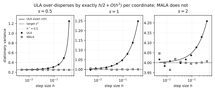
Three panels, one per scale s = 0.5, 1 and 2, of stationary variance against step size h on a log axis. ULA's measured variances (filled circles) follow the exact curve v(h) = s^2/(1 - h/2s^2), rising above the dashed target line s^2 as h grows; MALA's (open squares) stay near the target line. A dotted vertical line marks the stability limit h* = 0.5.

Figure 3. Gaussian stationary variance against the exact ULA law and target variance (the repository’s Figure 1). One panel per scale, $s = 0.5, 1, 2$ : the measured stationary variance against $h$ for ULA (filled circles) and MALA (open squares), the exact $v(h) = s^2/(1-h/2s^2)$ , the target $s^2$ (dashed) and the stability limit $h^* = 0.5$ (dotted). Anisotropic Gaussian, 128 chains × 200,000 steps per configuration. All 30 ULA cases lie within three estimated standard errors of $v(h)$ .

In the saved run, all 30 coordinate–step-size cases lie within three estimated variance standard errors of $v(h)$ , with relative standard errors from 0.11% to 0.85%. Near the limit the bias is large, and it is still where the formula puts it:

scale $s$	target $s^2$	ULA exact $v(h)$	ULA measured	MALA measured
0.5	0.25	1.25	1.2479	0.2494
1	1	1.25	1.2488	1.0003
2	4	4.2105	4.2085	4.0075

All at $h = 0.4$ , where MALA’s acceptance rate is 0.595.

Run It in the Browser

The widget below (Figure 4) runs one coordinate of that experiment in your browser. ULA acts coordinatewise, so a single coordinate is exactly one coordinate of the repository’s run. It moves 4,096 independent chains from a fixed seed, draws their histogram against $\mathcal N(0, s^2)$ (dashed) and $\mathcal N(0, v(h))$ (solid), and traces the ensemble variance against the step $k$ . For ULA the reference is exact at every step, not only in the limit. Iterating $v_{k+1} = a^2 v_k + 2h$ from $\operatorname{Var}(X_0)$ and subtracting the fixed point gives

\operatorname{Var}(X_k) = v(h) + a^{2k}\big(\operatorname{Var}(X_0) - v(h)\big), \qquad a = 1 - h/s^2,

an AR(1) identity derived from the update (it is not in the repository). Push $h$ past $2s^2$ and the formula has no stationary law to offer; the widget says so from the formula rather than waiting for the chains to overflow.

Figure 4. Classical baseline, run live: ULA and MALA on a one-dimensional Gaussian $\mathcal N(0, s^2)$ , with the repository’s update, closed form and acceptance rule, from a fixed seed. The readout compares the ensemble variance with the exact $\operatorname{Var}(X_k)$ (ULA) or with $s^2$ (MALA, valid in stationarity), in units of its independent-chain standard error. MALA’s acceptance rate here has no closed-form reference, and it need not match the repository’s 0.595 at $h = 0.4$ : that figure is for the three-coordinate target, where MALA accepts or rejects all coordinates jointly.

The Price of the Correction

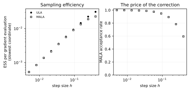
Removing the bias is not free. Figure 5 shows the bias rate: the measured $W_2$ proxy for ULA follows the exact first-order curve, while MALA sits at the Monte Carlo floor. Figure 6 shows the price, in effective samples per gradient evaluation and in MALA’s acceptance rate. Switch between the two with the dots above the figure.

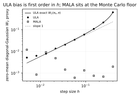
Log-log plot of the zero-mean diagonal-Gaussian 2-Wasserstein proxy against step size h. The exact ULA curve follows a dashed slope-1 reference line at small h and steepens toward the stability limit; the measured ULA proxy follows the exact curve except at the two smallest step sizes, where it sits above it; the measured MALA proxy scatters with no trend in h, at the Monte Carlo floor.

Figure 5. ULA bias is first order in $h$ ; MALA sits at the Monte Carlo floor. Log–log plot of the exact ULA $W_2(\pi_h, \pi)$ , the measured ULA and MALA proxies, and a slope-1 reference anchored at the exact value at $h = 0.005$ . The plotted estimates are zero-mean diagonal-Gaussian covariance proxies; they omit empirical mean and off-diagonal covariance errors. At the two smallest step sizes the ULA points sit above the exact curve (0.00513 measured against 0.00288 exact at $h = 0.005$ ). The repository reports no fitted slope; the evidence is the overlay.

Two panels. Left: effective sample size of the coordinate mean per gradient evaluation against h for ULA and MALA, for the slowest coordinate. Right: MALA's acceptance rate against h, falling from 0.999 to 0.595.

Figure 6. Mean ESS per actual gradient evaluation and MALA acceptance rate. Left: effective sample size of the coordinate mean per score evaluation, minimum over coordinates, ULA against MALA. Right: MALA’s acceptance rate against $h$ . ULA uses one score evaluation per step; MALA caches the current score and uses one per proposal plus one initial evaluation per chain. This is not a wall-clock comparison, and ULA’s effective samples are draws from $\pi_h$ , not from $\pi$ .

At $h = 0.4$ , ULA’s slowest-coordinate ESS per gradient is 0.0308 and MALA’s is 0.0225. Read next to Figure 3, ULA’s edge is in effective draws from $\pi_h$ , not from $\pi$ . In the repository’s words, “ULA’s error is a bias you cannot average away; MALA’s is a cost paid in rejected proposals.” The cost, across the sweep:

$h$	0.0050	0.0081	0.0132	0.0215	0.0351
MALA acceptance	0.9993	0.9986	0.9972	0.9942	0.9879
$h$	0.0570	0.0928	0.1511	0.2458	0.4000
MALA acceptance	0.9749	0.9480	0.8927	0.7835	0.5946

Rounded to four decimals from the saved values; the README rounds the end points to 0.999 and 0.595.

Results on a Two-Well Mixture

The second experiment asks what the correction does not fix. The target is an equal mixture of two Gaussians separated along the first coordinate $e_0$ ,

\pi = \tfrac12\,\mathcal N(-\mu e_0, s^2 I) + \tfrac12\,\mathcal N(+\mu e_0, s^2 I), \qquad \Delta(\mu) = \frac{\mu^2}{2s^2} - \log 2 ,

where $\Delta$ is a large-separation approximation to the barrier (the exact modes sit slightly closer to zero). Both samplers equilibrate rapidly within a mode and cross between modes on an exponentially longer timescale. Kramers-type asymptotics suggest a leading exponential $e^{-\Delta}$ , with a separation-dependent prefactor.

The run uses one step size, $h = 0.05$ , in two dimensions with $s = 1$ and $\mu$ from 2.0 to 5.0: 32 chains of 150,000 steps per separation, every chain started in the left well, sign crossings counted after a 20% burn-in (crossings during burn-in, or between steps, are not measured). The fit is $\log(\text{rate}) = c - b\,\Delta$ , compared with $b \approx 1$ , on separations with at least 20 crossings. That cutoff fits the two samplers on different supports: ULA through $\mu = 4.5$ (6 points), MALA through $\mu = 4.0$ (5 points).

The barrier law is asymptotic, so the fitted slope is a numerical comparison, not an exact transition-rate identity. Unlike the Gaussian experiment, there is no closed form here to grade against.

Figure 7. Two failure modes, two scalings. Left: ULA’s invariant law is wider than the target by $v(h) - s^2 = h/2 + O(h^2)$ , drawn at $s = 1$ , $h = 0.4$ ; the Metropolis step removes this in stationarity. Right: $-\log\pi$ along the line through both modes, drawn exactly for $\mu = 3$ , $s = 1$ . The crossing rate falls like $e^{-\Delta}$ to leading order, and the Metropolis step does not remove that here. Correcting discretization bias does not by itself ensure rapid mixing.

Figure 8 shows the measurements in the repository’s own figure: the time each sampler spends in the right well, and how often it crosses, as the approximate barrier grows.

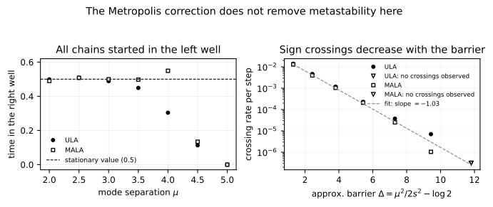
$Two panels. Left: fraction of time in the right well against separation mu for ULA and MALA, with every chain started in the left well and the stationary value 0.5 dashed; occupancy stays near 0.5 at small separations and falls to 0 by mu = 5. Right: sign-crossing rate per step against the approximate barrier Delta on a log scale; the points fall roughly along a dashed fitted line of slope -1.03, and triangles at Delta = 11.8 mark the separation with no crossings observed, drawn at a plotting floor.$

Figure 8. Well occupancy and sign-crossing rates as the approximate barrier grows (the repository’s Figure 4). Left: fraction of time in the right well against $\mu$ ; every chain starts in the left well, and the stationary value 0.5 is dashed. Right: sign-crossing rate per step against $\Delta$ , log scale. The dashed line is the MALA fit (slope −1.03), drawn across the whole $\Delta$ range and therefore extrapolated beyond its $\mu \le 4$ support. The “no crossings observed” triangles at $\Delta = 11.8$ are drawn at an arbitrary plotting floor, $1/(n_{\text{chains}} \times 10^5)$ ; they are not a measured rate.

Fitting $\log(\text{crossing rate})$ against $\Delta$ gives slope −0.948 for ULA ( $R^2 = 0.998$ ) and −1.032 for MALA ( $R^2 = 0.999$ ), near the leading exponential’s slope −1. Because the supports differ, the two slopes should not be read against each other to three digits.

sampler	slope	$R^2$	points used	$\mu$ used
ULA	−0.948	0.998	6	2.0 to 4.5
MALA	−1.032	0.999	5	2.0 to 4.0

Crossings by separation, for 32 chains at $h = 0.05$ after a 20% burn-in:

$\mu$	$\Delta$	ULA crossings	ULA chains never crossed	MALA crossings	MALA chains never crossed
2.0	1.31	53820	0	50091	0
2.5	2.43	17967	0	15250	0
3.0	3.81	4565	0	3996	0
3.5	5.43	886	0	802	0
4.0	7.31	144	5	96	6
4.5	9.43	27	21	4	28
5.0	11.81	0	32	0	32

At $\mu = 5$ ( $\Delta = 11.8$ ) neither sampler crosses during the measured window, and all 32 chains of each stay in the well they started in. A zero count bounds a rate rather than measuring it, so that row is a detection limit, not a further point on the line. Nor does MALA’s guarantee reach this regime: it is unbiased in stationarity, but a chain trapped near its initial well is nowhere near stationarity. One difference the repository leaves open: at $\mu = 4.5$ ULA records 27 crossings to MALA’s 4, and the study does not test why.

Dynamics, Not Only the Invariant Law

A sampler can get the invariant measure right and still get the dynamics wrong. For a one-dimensional periodic potential the long-time diffusivity has an exact value, given by the classical Lifson–Jackson formula (a textbook benchmark, not a result of this project) with free diffusivity $D_0 = \beta^{-1}$ and averages over one period:

D_{\mathrm{eff}} = \frac{D_0}{\langle e^{\beta V}\rangle\,\langle e^{-\beta V}\rangle}, \qquad V(x) = \cos x,\ \beta = 1:\quad D_{\mathrm{eff}} = I_0(1)^{-2} = 0.6238603604\ldots

Any Langevin integrator has to reproduce it as the step size shrinks. As this site puts it, “One that gets the invariant measure right and the diffusivity wrong has a bug in its time discretization.” Figure 9 runs the textbook mean-squared-displacement estimator live, with 1024 replicas at $\beta = 1$ and $h = 0.01$ . The site’s check script, run at longer time, measures $\hat D(2000) = 0.6218$ with a standard error of 0.0098.

Fig. 9. Effective diffusivity in the cosine potential, β = 1, 1024 independent replicas, Euler–Maruyama at h = 0.01. The dashed line is the Lifson–Jackson value D_eff = 1/I₀(1)² = 0.6238603604…, computed from the Bessel series and cross-checked against quadrature. Nothing here is fitted, and the trace is unsmoothed: the residual at t = 1000 is the transient, not Monte Carlo error, and the band is ±1 s.e. across four disjoint replica groups.

The band in Figure 10 is the same dynamics in two dimensions, $dX_t = -\nabla V(X_t)\,dt + \sqrt{2\beta^{-1}}\,dW_t$ with $V(x,y) = \cos x + \cos y$ on the torus, $\beta = 2$ and $h = 0.004$ . It is checked against its Gibbs law through $\mathbb E_\pi[\cos X] = -I_1(\beta)/I_0(\beta)$ . The site’s check script recorded total-variation distances $\mathrm{TV}_{1D} = 1.021\times10^{-3}$ and $\mathrm{TV}_{2D} = 3.945\times10^{-3}$ (measured 2026-07-30), and a discretization bias in $\mathbb E[\cos X]$ at the shipped step of $9\times10^{-4} \pm 4\times10^{-4}$ (one standard error), barely resolved from zero.

Figure 10. Overdamped Langevin dynamics in $V(x,y) = \cos x + \cos y$ at $\beta = 2$ , Euler–Maruyama at $h = 0.004$ , running live in your browser. Particles collect in the potential wells, where the Gibbs measure $\propto e^{-\beta V}$ concentrates, and occasionally hop between neighboring wells; color encodes the local potential energy.

The third live figure (Figure 11) is a related sampler from generative modeling. It runs a diffusion model’s reverse-time sampler with the exact score of a Gaussian mixture, so it can be graded on mode coverage rather than on how plausible its samples look; its caption gives the setup and the grade. It is the reverse-time update, not the Langevin corrector of Figure 1, and like Figures 9 and 10 it lives in this site’s code, not in langevin-samplers.

**Fig. 11.** Ancestral sampling from a continuous-time diffusion model. The forward variance-preserving SDE noises a six-component Gaussian mixture into 𝒩(0, I); the reverse SDE carries 640 samples back over 320 Euler–Maruyama steps. Because a mixture stays a mixture under the VP kernel, the score used here is exact rather than learned, which leaves discretization as the only source of error and turns the mixture weights into something gradable. True weights (0.28, 0.22, 0.17, 0.14, 0.11, 0.08); the readout reports max_k |ŵ_k − w_k| at the end of each pass, against a Monte Carlo floor of 0.018 at n = 640. Color and contours encode −log p₀.

Ongoing Work: Molecular Systems

With Dr. David Herzog, Department of Mathematics, Iowa State University, we have drafted a manuscript, Langevin Dynamics and Transport-Coefficient Estimation for Molecular Systems, which is now in his review. The work develops samplers for overdamped Langevin dynamics “staged from a 1D periodic potential up to a solvated ion in a 3D Lennard-Jones bath,” and uses them to estimate transport coefficients: the long-time constants, such as a diffusion coefficient, that describe how particles move rather than where they sit at equilibrium.

This is why the previous section matters. A sampler can reproduce the invariant law and still get the dynamics wrong, and a transport coefficient is a property of the dynamics, so an equilibrium check alone does not test it. Everything else on this page draws only on the public repository, this site’s live figures and textbook results; it shows none of the manuscript’s methods or results.

Status

The draft is in advisor review with Dr. Herzog. Its methods and results are held back pending submission.

Conclusion

Dropping the Metropolis step costs a bias, first order in the step size, that sits where the closed form puts it. Keeping the step removes the bias at a price in rejected proposals, but it does not by itself ensure rapid mixing. The answers, in brief:

Question	What the saved runs and checks show
Does ULA’s measured variance agree with the exact law $v(h)$ ?	In all 30 coordinate–step-size cases, within three estimated standard errors (relative SEs 0.11% to 0.85%)
How large is the bias near the stability limit, $h = 0.4$ with $h^* = 0.5$ ?	Measured [1.2479, 1.2488, 4.2085] against exact [1.25, 1.25, 4.2105], for targets [0.25, 1, 4]
What does the Metropolis step buy, and at what price?	MALA returns [0.2494, 1.0003, 4.0075]; its acceptance falls from 0.999 to 0.595 over the sweep
Does it fix slow mixing between modes?	Not here. Log crossing rate against the barrier: slope −0.948 (ULA, fitted on $\mu \le 4.5$ ) and −1.032 (MALA, fitted on $\mu \le 4.0$ ), near the leading exponential’s −1
Are the dynamics right, not only the invariant law?	The site’s check script (not the repository) measures $\hat D(2000) = 0.6218$ (s.e. 0.0098) against the Lifson–Jackson value 0.62386

These results cover ULA and MALA with exact scores only. The machine-learning samplers in the dashed boxes of Figure 1 are this site’s framing, and nothing here tests them.

Reproduce

The repository figures and the saved results behind the experiment tables come from langevin-samplers (MIT). Its README gives these commands:

uv sync
uv run python -m unittest discover -s tests -v
uv run python scripts/01_gaussian_bias.py --smoke   # ~10s pipeline check
uv run python scripts/01_gaussian_bias.py
uv run python scripts/02_multimodal.py
uv run python scripts/03_plot.py

Runs are seeded, with streams keyed by role and configuration, and each writes a sidecar that records its seed, parameters and commit. GitHub Actions runs the regression suite and a small end-to-end pipeline on every push and pull request, and the AR(1) uncertainty test compares predicted variance standard errors with the actual spread across independent simulated experiments.

Settings

Experiment	Settings, as in the scripts
Gaussian bias (`scripts/01`)	seed 20260729; scales 0.5, 1, 2; 10 log-spaced $h \in [5\times10^{-3}, 0.4]$ ; 128 chains × 200,000 steps, thin 20, burn-in 20%; start: standard normal × 2
Metastability (`scripts/02`)	$s = 1$ , dimension 2, one step size $h = 0.05$ ; $\mu$ from 2.0 to 5.0; 32 chains × 150,000 steps, thin 1, burn-in 20%; all chains start in the left well; fits on separations with at least 20 crossings

Provenance

The two saved results come from different commits, as their sidecars record. The validation sidecar also hashes the result file it checked.

Result file	Commit	Run
`results/gaussian_bias.json`	`6ee068e`	2026-10-26, macOS, Python 3.14.7
`results/multimodal.json`	`9c18b87`	2026-07-30, Windows, Python 3.12.10

Layout

src/langevin/     library
  targets.py      Gaussian and two-component mixture (score + reference moments)
  samplers.py     ULA and MALA, vectorized over independent chains
  theory.py       exact ULA stationary law, stability limit, Gaussian W2
  diagnostics.py  Geyer ESS for means, pooled moments, independent-chain variance SE
  provenance.py   run sidecars (parameters, seed, resolved commit SHA)
scripts/          01 gaussian bias -> 02 multimodal -> 03 figures
results/          JSON outputs + .meta.json sidecars
figures/          PDFs and PNGs
tests/            analytic sampler, accounting, uncertainty-calibration and provenance checks

Code Back to the demo

References

The repository’s reference list.

Roberts, G. O. and Tweedie, R. L. (1996). Exponential convergence of Langevin distributions and their discrete approximations. Bernoulli 2(4), 341–363.
Roberts, G. O. and Rosenthal, J. S. (1998). Optimal scaling of discrete approximations to Langevin diffusions. JRSS-B 60(1), 255–268.
Dalalyan, A. S. (2017). Theoretical guarantees for approximate sampling from smooth and log-concave densities. JRSS-B 79(3), 651–676.
Durmus, A. and Moulines, É. (2017). Nonasymptotic convergence analysis for the unadjusted Langevin algorithm. Annals of Applied Probability 27(3), 1551–1587.

Inside the Trap All research Rare Events