Akshat Valse · stochastic foundations of machine learning

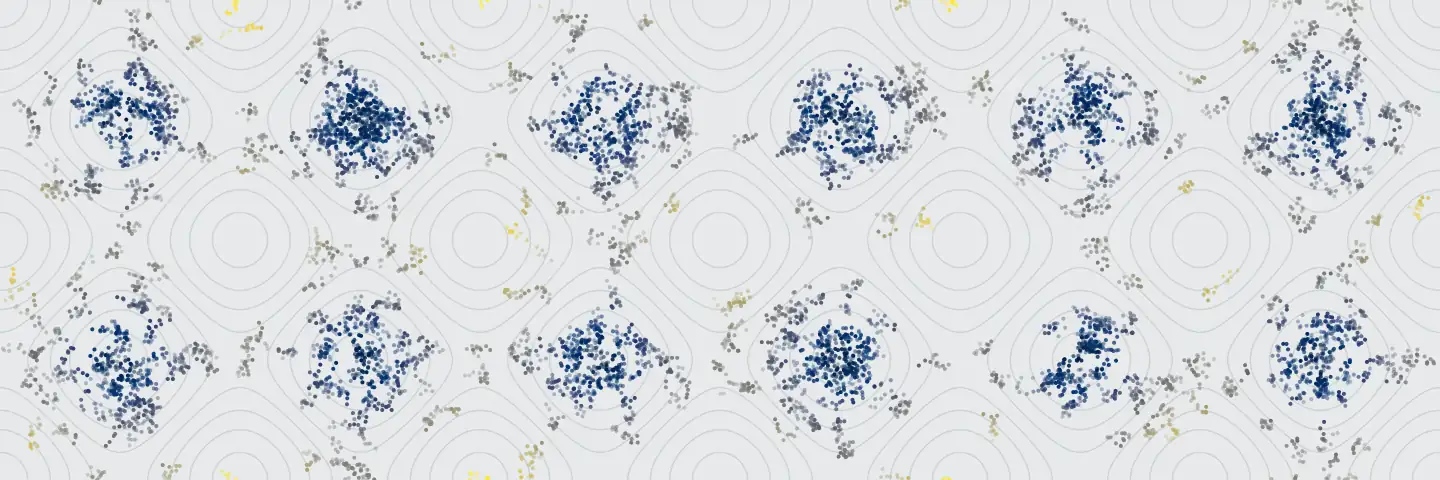
Fig. 1

object: overdamped Langevin
potential: V = cos x + cos y
integrator: Euler–Maruyama, h = 0.004
checked: TV 1.0×10⁻³ vs Gibbs

colour: V

I work on the stochastic foundations of machine learning: the theory of stochastic differential equations, applied to the algorithms that now generate and sample. A diffusion model is a reverse-time SDE, stochastic gradient descent and its Langevin variants are diffusions in a rough loss landscape, and a PAC-Bayes bound is the Donsker–Varadhan formula applied to a posterior over hypotheses. Three questions occupy me: what the discretisation of a Langevin sampler actually costs, how to estimate probabilities too small for direct simulation to reach, and whether a PDE solver with a network inside it will hold together when you iterate it. Underneath all three is the same question, which is what can be proved about the objects practitioners already use: rates, stability, and error bounds in place of heuristics. Everything moving on this page is one of those objects, running live and graded against a closed-form answer.

The band above is running in your browser from a fixed seed. It integrates

d X_{t} = - \nabla V (X_{t}) d t + 2 β^{- 1} d W_{t}

on the torus. Annealed Langevin sampling runs this same dynamics at each noise level, and it is the continuous-time limit of SGLD when

V

is the loss. Replace

\nabla V

by a learned score and you have a generative model. Because the score here is exact, the answer can be checked. Particles collect where

e^{- β V}

is large and hop between wells at the Kramers rate, and across 48 bins the empirical measure sits within a total variation of

1.0 \times 1 0^{- 3}

of the Gibbs law, with a discretisation bias of

9 \times 1 0^{- 4}

on

E [cos X]

against the closed form

- I_{1} (β) / I_{0} (β)

.

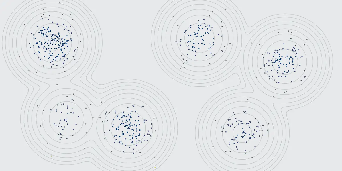
Fig. 2

object: VP-SDE, reverse time
score: exact, not learned
steps: 320 Euler–Maruyama
graded on: mode coverage

A diffusion model with an answer key

Generative models are hard to evaluate because the target is unknown, so a sampler can only be judged on whether its output looks plausible. Make the target a Gaussian mixture and that changes. The mixture is closed under the variance-preserving forward kernel, so every marginal $p_{t}$ is again a mixture and the score $\nabla lo g p_{t}$ is available in closed form. Anderson's time reversal

d X = [- \frac{1}{2} β (t) X - β (t) \nabla lo g p_{t} (X)] d t + β (t) d \overset{ˉ}{W}

then runs with an oracle score, so whatever error remains belongs to the sampler and not to a network. The weights below are deliberately unequal, which is what makes mode collapse detectable at all. A sampler that drops the 0.08 component still emits individually plausible points, and only the proportions give it away.

**Fig. 2.** Ancestral sampling from a continuous-time diffusion model. The forward variance-preserving SDE noises a six-component Gaussian mixture into 𝒩(0, I); the reverse SDE carries 640 samples back over 320 Euler–Maruyama steps. Because a mixture stays a mixture under the VP kernel, the score used here is exact rather than learned, which leaves discretisation as the only source of error and turns the mixture weights into something gradable. True weights (0.28, 0.22, 0.17, 0.14, 0.11, 0.08); the readout reports max_k |ŵ_k − w_k| at the end of each pass, against a Monte Carlo floor of 0.018 at n = 640. Colour and contours encode −log p₀.

Over 16,384 samples the recovered weights match to $max_{k} ∣ \overset{w}{^}_{k} - w_{k} ∣ = 0.006$ against a Monte Carlo standard error of $0.0035$ , the component means to $0.010$ , and the within-component spread to $0.262$ against $σ = 0.26$ . This is what a toy target with a closed form buys you. The sampler either returns the weights or it does not, and no quantity of plausible-looking output makes up the difference. The full check is here.

research

Research

Langevin dynamics: sampling, discretisation bias, transport coefficients

David Herzog · Mathematics · ongoing

The sampler underneath score-based generative models and stochastic-gradient Langevin dynamics, analysed where its errors are computable: discretisation bias against exact stationary laws, and estimator design for effective diffusivity and mobility.

Large-deviation asymptotics for mean-field interacting systems

Ruoyu Wu · Mathematics · ongoing

Rate functionals and the variational characterisation of rare events for the empirical measure of a mean-field particle system. This is the construction that sits one level above the mean-field limit of wide-network training, and the machinery underneath PAC-Bayes.

Stability certificates for neural PDE solvers

Jue Yan · Mathematics · ongoing

Trained solvers with indistinguishable loss diverge or survive under long rollouts. A frozen-state von Neumann analysis of the learned update predicts which, and yields a learned analogue of the CFL condition.

Full descriptions →

notes

Notes

Grading a diffusion model when you know the answer Jul 2026
A Gaussian mixture is closed under the variance-preserving forward kernel, so the score is exact and the sampler can be marked on mode coverage rather than judged on whether its output looks plausible.
Effective diffusivity in a periodic potential Jul 2026
How fast does a Langevin sampler actually explore a rough landscape? In one periodic dimension the answer is exact, 1/I₀(β)², which makes it a benchmark a sampler either reproduces or fails.
What the Metropolis correction buys, and what it does not Jul 2026
The unadjusted Langevin algorithm is SGLD without the minibatch noise. On a Gaussian target its stationary law is exact, so the bias can be measured against a formula, and a metastable target then shows that removing the bias does nothing for the harder problem.

elsewhere

Elsewhere

email: avalse@iastate.edu
github: AkshatValse
cv: /cv

Preprints will be posted here as they become available.